LCTR / CONSTRUCTING TIME
How to Create TimeBuilding time and descriptions of change from a counter, records, a switch, and information coupling
LCTR (Local-comparison theory of time reference) constructs time from physical counting, records, differences in object states, and information coupling. This page uses three records retained by one apparatus to construct temporal identity, order, numerical representations, and a representation of object states, step by step. By the end, the switch state can be written as a function of a time variable.
1. Specify what the components supply
Consider an apparatus with one counter, one memory, one switch, and one coupling circuit.
The four role symbols , , , and are the initials of Clock, Detector, Body, and Observer, respectively.
| LCTR role | Component in this example | Assigned function |
|---|---|---|
| : clock side | Counter | Distinguish internal count positions and supply their ordering under updates |
| : record side | Memory | Retain correspondences between counter inputs and switch-state inputs and make them available for readout |
| : object-state side | Switch | Supply the difference between open and closed states |
| : observer-side information coupling | Coupling circuit | Identify connected inputs and bind corresponding counter inputs, records, and state inputs |
The record-side role integrates detection, recording, and re-presentation; LCTR uses Detector as the representative term for this role.
We now look inside the counter that fulfills the role in the table. Attach a distinguishing label to each of its count positions. The labels used in this explanation are a red circle ●, a blue triangle ▲, and a green diamond ◆. Each label has a color, a shape, and a name, and identifies a distinct count position.
Use these labels to follow how the four roles contribute to one record. In this example, pair the red-marked counter input with a switch input having state Closed, and retain that correspondence in memory.
- The counter in clock-side role supplies the input originating at the position marked with a red circle ●.
- The switch in object-state role supplies an input having state Closed.
- The coupling circuit in information-coupling role binds the specified counter input and switch input to the record that retains their correspondence.
- The memory in record-side role retains this correspondence. Give this record the name Card A.
Reading Card A’s counter field identifies the red-marked input on the side; reading its switch field identifies the Closed input on the side. Card A itself is the record on the side, while binds the respective inputs to that record. The blue triangle ▲ and green diamond ◆ label other distinct count positions within the same counter. The next section pairs the inputs from these positions with separate cards.
Give this counter an update rule that maps the red-marked position to the blue-marked position and the blue-marked position to the green-marked position. Chaining these correspondences, as one would follow the arrows in the diagram, also connects the red-marked position to the green-marked position. The color names identify positions, while the update rule supplies relations between positions. The connections specified by this rule provide the basis for comparison here.
The counter’s full source includes count positions beyond those shown in this explanation. Give those positions their own distinct labels as well. The diagram selects only the records originating at the red, blue, and green positions. Specify the count-position relation supplied by the update rule, the time representation constructed later, and its correspondence to seconds at their respective stages.
Correspondence with the paper’s input type. This counter displays each natural-number count position used in the paper with its own distinct label. The red mark denotes the designated starting position, the blue mark its update target, and the green mark the update target of blue. For the other positions, specify update targets according to the successor relation of counting in the paper. The correspondence with these labels identifies positions one-to-one, preserving the distinctions between count positions and their comparison relation.
In the steps below, we identify the original inputs from the apparatus’s readouts. We then group the inputs treated as the same under the construction rules. We similarly group the switch-side inputs and use the correspondences retained in the records to relate the groups obtained on the two sides. LCTR uses these materials to construct a temporal structure that supports comparison.
The four symbols denote roles. A “carrier” is a physical entity that realizes such a role; the counter and memory are examples here. A configuration in which one carrier realizes several roles can also be considered. To determine the required number of objects, specify how each role is realized and what counts as one object.
2. Make three records
To identify inputs on the clock side , specify the physical counter, its internal update rule, the red-marked position as its starting position, and its connection to the record side . This determines the configuration supplying the inputs. The LCTR paper calls the physical provider of count positions and updates a “source.” Give this source the identifying name .
Another counter can also carry a red label. To identify which counter supplied the input, retain the origin “red-marked position of source K” in the record. The combination of label and source allows the readout to identify the relevant position of this counter.
Write the inputs originating at the red, blue, and green positions of this counter as , respectively. Each subscript names the color of the position from which the input originates. The diagrams retain the color and shape of each input.
The memory in record-side role uses Card B and Card C as identifying labels alongside Card A introduced above. Each card denotes one record. First, the coupling circuit fulfilling specifies the storage location for Card A. The counter readout passes “red-marked position of source K” to that card’s counter field. The readout of the switch fulfilling passes the switch specification, input identifier, and state Closed to the state field of the same card. The coupling circuit binds these items as the correspondence retained in Card A.
Give the switch input passed to Card A the identifier . The memory retains the card’s content and identifying label A. Write this record individual as . The readout rule returns the original input names and content from Card A.
Card B pairs the blue-marked input with a switch input having state Open; Card C pairs the green-marked input with a switch input having state Closed.
| Record label | Origin retained in the counter field | Switch-input identifier | State-field value |
|---|---|---|---|
| Card A: | Red mark ● of K: | Closed | |
| Card B: | Blue mark ▲ of K: | Open | |
| Card C: | Green mark ◆ of K: | Closed |
Reading Card A reveals that the input originating at the red-marked position of source K corresponds to input of the specified switch, whose state value is Closed. The memory uses a separate storage location for each card and identifies each record by its content and identifying label. The correspondence between the label Card A and the red mark can be checked from the content retained by the coupling circuit.
Card A and Card C both retain Closed. One is linked to the red-marked input, and the other to the green-marked input. Their switch-input identifiers are also distinct: and . Inputs with the same state value remain in separate records. This distinction will be used to represent changes in the object.
- Red position
- Blue position
- Green position
- Record label: Card A
- Equivalence class: a set containing inputs
- Order coordinate
- Name of the real value assigned at the final step
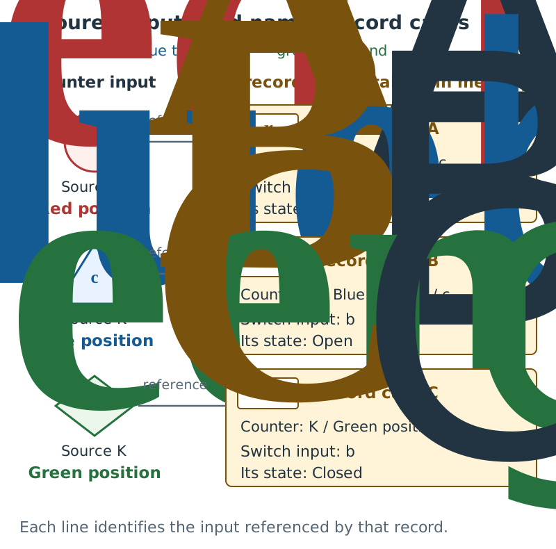
Distinguishing inputs and records
The memory fulfilling D retains cards pairing inputs from the C counter with inputs from the B switch. The O coupling circuit binds these inputs to their records. The red circle cred, blue triangle cblue and green diamond cgreen identify inputs from distinct positions of source K. The records retained in memory are Card A (rA), Card B (rB), and Card C (rC). Each card has separate entries for the counter field, switch-input name and state value. Each line shows which counter input the card references.
Cards A and C both contain Closed. Retaining input identifiers and origins distinguishes the red input from the green input, and switch input bA from bC.
3. Identify the original inputs from the readouts
Specify a coupling circuit, the range of inputs it receives, the input-identification rules, and the comparison rules for the checks. This example performs its checks under that configuration. The paper’s “reception context” is a configuration of this kind, specifying a receiving carrier together with the inputs and relations it handles.
Read Card B. Its counter field, “blue-marked position of source K,” identifies the blue input . The switch specification and input name in its switch field identify ; the record content and card label B identify the record itself as . These are the input-recovery rules for this example.
When checking counter inputs against records, examine which of Cards A, B, and C corresponds to the red input. Card A’s counter field retains the red-marked origin, while Card B retains the blue-marked origin. Reading this content identifies Card A as the record corresponding to the red input. Check the other colors in the same way.
Give the collection of correspondences retained in the records the name .
Each parenthesized pair contains one counter input and one record. For example, the pair , consisting of the red input and Card B, does not match the blue mark retained by Card B. This pair is not included in .
For the comparison rules in this example, use identity rules mapping each identified input to itself. Specify this rule for the clock side, the record side, and their pairs. Applying it to the red input paired with Card A returns that same pair. Applying it to the red input paired with Card B also returns the same pair, retaining the mismatch with the record content. The comparison rule is specified separately from any operation that would create a correspondence by renaming inputs.
Also specify the order relations used for comparison. On the clock side, use the relation red mark → blue mark → green mark supplied by the counter’s update rule. On the record side, use the separately specified relation Card A → Card B → Card C in memory. The letters identify records; the relation specified in memory determines this direction. Use the card labels as a one-to-one display of the internal record indices included in the paper’s record inputs, preserving the comparison relation specified on those indices. On each side, include self-pairs and pairs obtained by chaining the relation.
| What to check | Calculation or verification in this example |
|---|---|
| Is the original input uniquely determined? | The source and color label, the record content and card label, and the switch specification and input name identify the respective inputs |
| Does the joint rule agree with the separate rules? | Returning a pair unchanged gives the same result as returning each input unchanged and pairing them |
| Does combining the rules preserve the corresponding input? | Combining identity rules still maps every input to itself |
| Is the correspondence retained by the records preserved? | Every pair in maps to that same pair |
| Does the choice of an input treated as the same preserve order? | Under this example’s identification rule, each group contains just one input |
| Can order coordinates be constructed? | The relations specified on the clock and record sides determine the direction of comparison for every pair of distinct inputs considered. With one reception context, the global construction combining them uses the same order |
In general, when a group of inputs treated as the same contains several inputs, one of them is selected for a calculation. The selected input is called a “representative.” The order judgment must agree whichever representative is selected. In this example, each group contains one uniquely determined input.
Chapter 4 of the paper expresses the establishment of comparison and order under the specified conditions as . Here comprises the inputs and rules used for comparison. Alongside the color and record labels, the recovery, comparison, and order rules specified above support this example’s construction.
4. Group inputs treated as the same
Each card retains a correspondence between a counter input, the record itself, and a switch input. For example, write the content of Card B as
Here is an identifying name for this correspondence. Give the correspondences for Card A and Card C the names , respectively.
Also specify a rule binding these correspondences to one another. In this example, bind each card’s correspondence to itself. For Card B, this gives . Bind no correspondences from different cards. A correspondence retained within a card’s fields and the rule binding cards’ correspondences to one another are separate specifications.
Recover the original inputs from the coupling circuit’s receptions, and extract the counter-side input from each of the two bound correspondences. For Card B, this gives
The resulting pair contains the blue input and that same blue input. Apply the same operation to red and green.
In mathematics, a collection of input pairs is a “relation.” Include each input paired with itself, the reverse of each pair, and pairs obtained by chaining pairs. These properties are called reflexivity, symmetry, and transitivity, respectively. Retaining the original pairs and adding every pair required by these rules gives the smallest such relation, called the reflexive, symmetric, and transitive closure.
Check the blue pair. Reversing gives the same pair; chaining this pair with itself also gives a pair of blue with blue. Collecting the inputs treated as the same as blue therefore collects only the blue input in this example. Red and green each give the corresponding result.
The resulting sets of inputs are called equivalence classes in mathematics. The diagrams use purple enclosures and show each member input inside its enclosure with its colored mark.
Compare the blue triangular input with the purple enclosure . The former denotes one input; the latter denotes a set containing that input. Although this set has a single member in the example, the input itself and the set containing it are distinct objects.
A set whose elements are equivalence classes is called a “quotient set.” A quotient set allows each group of inputs treated as the same to be passed to the next operation as one element. In general, when several inputs are grouped, check that subsequent operations give the same result whichever input is selected as a representative.
The LCTR paper defines the set of clock-side input equivalence classes as the “observer-time quotient,” written as
Here is the clock-side source-input set, is the identification relation just constructed, and is the observer-side information-coupling position. The red, blue, and green equivalence classes are elements of this observer-time quotient. For inputs not included in the records, the rule that includes each input paired with itself also yields an equivalence class containing that input alone.
5. Establish order and represent time numerically
The pair connecting the red and blue marks under the counter’s update rule corresponds to the equivalence-class pair . The blue–green pair likewise corresponds to . Include self-pairs and pairs obtained by chaining the relation.
Write the comparisons holding between distinct equivalence classes as . In this example,
Chaining the red–blue and blue–green relations also gives the red–green comparison. Specifying the rule for grouping inputs as the same separately from the relation used to establish this order determines the direction of comparison while preserving the distinction between inputs.
In a general construction, the order relation may hold in neither direction between two equivalence classes. “Transitive incomparability” means that if one class cannot be compared with another, and that other class cannot be compared with a further class, then the classes at the two ends cannot be compared either. Under this condition, LCTR groups incomparable classes to form order coordinates. The paper defines the resulting set as the “observer-time order-coordinate quotient.”
Section 4 constructed equivalence classes from the original inputs. Here, the resulting equivalence classes are grouped further according to order. The count positions in this example are comparable under the specified update relation. The red, blue, and green equivalence classes correspond to separate order coordinates, written as . The diagrams show them in gray rectangular frames.
Next, choose a map that represents this order by the relative sizes of real numbers. Give the real values that it assigns to the red, blue, and green coordinates the names τ-red, τ-blue, and τ-green, respectively. In formulas, write them as . The chosen map preserves order, so these values satisfy
Names such as τ-red denote the real values assigned at this stage. The red mark and the other initial labels identify positions of source K. The diagrams distinguish these roles through colored marks and orange numerical-display frames.
Follow the blue row in detail. Purple is the set containing the blue input; gray is its order coordinate; orange is the value the chosen map assigns to that coordinate.
| Label identifying the original input | Equivalence class containing the input | Its order coordinate | Name of the assigned real value |
|---|---|---|---|
| Red ●: | τ-red: | ||
| Blue ▲: | τ-blue: | ||
| Green ◆: | τ-green: |
A “map” is a rule assigning exactly one output to each input. Here, combine the map from equivalence classes to order coordinates with the map assigning real values to those coordinates. This combination is called a composite map. The paper’s “law-admissible time representation” is constructed as
The symbol specifies that the operation on the right is performed first. For blue,
Passing from the equivalence class to its coordinate and assigning a real number to that coordinate yields the time representation corresponding to blue.
Other real-number representations preserving the same order can also be chosen. Choosing a different representation preserves the order while changing the assigned real values. Treating time intervals as physical quantities or expressing them in seconds requires further quantitative structure and a correspondence to units.
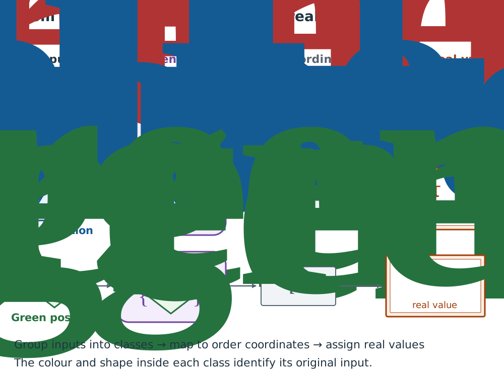
From inputs to classes, coordinates and real values
Follow the middle row. The blue triangle cblue is one input. Purple enclosure Tblue is the set {cblue} containing that input. This set maps to gray order coordinate [Tblue], and the chosen map assigns a real value to that coordinate. The symbol τblue on the right names the assigned real value.
From left to right, the arrows mean: find the equivalence class containing the input; map that class to its order coordinate; assign a real value using the chosen map. Following the color and shape along each row identifies the correspondence originating from the same input.
6. Express the switch state as a function of time
On the switch side, construct an identification relation using the same binding rule as in Section 4. Group the switch inputs corresponding to Cards A, B, and C into their respective equivalence classes:
The brackets in denote the set of inputs treated as the same as input under the switch-side identification relation. In this example, the only member of this set is itself. These equivalence classes are elements of the paper’s “object-state quotient.”
Card A supplies the correspondence between the red input and switch input . Passing both sides to their equivalence classes gives . The same operation gives from Card B and from Card C. These correspondences form this example’s trajectory relation.
Each clock-side equivalence class specified by the three records corresponds to one switch-side equivalence class. Each class has one uniquely determined input, and passage to order coordinates merges no distinct clock-side classes. We can therefore construct a function returning one switch state for each specified time-representation value.
Use the state names Closed and Open directly as readout values. Read Closed from and , and Open from . Reading the same input returns the same state name, and the example uses this readout consistently within its reception context.
| Record retaining the correspondence | Generated time representation | Corresponding switch-input equivalence class | State readout |
|---|---|---|---|
| Card A | τ-red: | Closed | |
| Card B | τ-blue: | Open | |
| Card C | τ-green: | Closed |
Use the row for Card C to construct one state representation. On the clock side, the equivalence class containing the green input is assigned the time-representation value τ-green. On the switch side, the same card specifies , whose readout is Closed. Through the correspondence retained in the card, specifying τ-green returns Closed. Write this correspondence as .
Applying the same operation to the other cards gives
The value in parentheses is a real value of the constructed time representation. The right-hand side of the equals sign is a switch-state name. τ-red and τ-green denote distinct time-representation values, and both correspond to the same state name, Closed.
Conversely, specifying τ-green and tracing the original correspondence gives the order coordinate . The time-representation map preserves order and assigns distinct real values to distinct coordinates, so the corresponding coordinate is uniquely determined. Following the trajectory relation from there and reading the state of returns Closed.
The “image” of a map is the set of values it actually assigns to its full specified input set. The rule recovering the original order coordinate from such a value is the “inverse map on the image.” The paper writes this rule as .
The set of values that a function accepts as inputs is its “domain.” The records with specified states here are Cards A, B, and C, so the domain of is the set consisting of τ-red, τ-blue, and τ-green. Among the possible time-representation values for the full counter, this set comprises the values for which a state representation has been supplied.
Choosing a different map for the time representation leaves unchanged which switch input and state name each card retains. The state representation can be reconstructed by pairing each new representation value with the state name in the same card.
7. What is needed for seconds, continuous curves, differentiation, and physical laws?
The construction has yielded temporal identity, order, a real-valued time representation, and a time-dependent representation of object states. When quantities or continuous representations are needed, add structure appropriate to their intended use.
To treat time differences as physical quantities, specify quantitative structure supporting the comparison and addition of differences, together with its conditions of validity. To express them in seconds, establish a correspondence between the generated time representation and the unit. This additional construction gives the counter-derived relation meaning in terms of physical intervals or units.
The state field in this example retains the distinction Closed/Open. To proceed, for example, to a model treating the distance between switch contacts as a continuous quantity, specify a distance readout, a scale for comparing its values, units, and tolerances, and connect that readout to the original inputs and records. Supplying this quantitative structure alongside the distinction between state names provides the materials for considering a continuous curve.
“Interpolation” selects a rule that agrees with the values at given points and assigns values between them. In a model with numerical samples, construct interpolation candidates and examine which physical quantity their values approximate, over which domain, and to what accuracy. Retain the state names Closed and Open used here as distinctions between switch states.
Using a continuous approximation requires specifying a scale and tolerances, then evaluating count steps, record stability, record-cell width, typed-record separation, object-state discrimination, and information-coupling limits. Typed-record separation checks elements of the observer-time quotient, elements of the object-state quotient, and their correspondence pairs: within each type, do the record images keep distinct entities distinguishable? Also check fit to the finite sample, continuous extension, and stability of order and relations.
Even a continuous curve may have a corner where the tangent slope is not uniquely defined. At the stage of using differentiation, check that the required derivatives exist wherever they are needed. Thus, the conditions for using a continuous representation and those for using a differential formulation are checked separately.
To use generated time in a physical law, keep the law’s domain of use within the generated trajectory’s time domain, and check applicability, uniqueness of outputs, satisfaction of the law relation, preservation of that relation under faithful representation changes, and a nonempty, admissible common valid domain for multiple laws. Once law-time admissibility is established, proceeding to a differential formulation also requires checking coordinate-system regularity, existence of the required derivatives, membership of derivative data in the law relation, and preservation of that relation under changes of value coordinates and time representation. Chapters 5 and 6 of the paper formalize these additional conditions and their failures.
“Satisfaction of the law relation” means that the constructed quantities satisfy the conditions specified by that physical law. The “common valid domain” is the intersection of the valid domains of the laws being combined. “Nonempty” means that this intersection contains at least one element. In addition to checking that there is a common element, check that this domain satisfies the admissibility conditions specified for using the laws together.
8. Break the construction and identify what goes wrong
First, consider discarding the switch-input identifier and receiving only Closed at the stage of recovering the original input. Both , corresponding to Card A, and , corresponding to Card C, have the state value Closed. Retaining only the state name prevents unique identification of the input from which the reception originated. The problem occurs at the stage of recovering the original input from a switch-side reception.
In the original construction, Card A could be traced to the red input and Card C to the green input. Reading while preserving those correspondences gives the state representation Closed at τ-red and Closed at τ-green. The same state name can be used while distinguishing the input and time representation to which it corresponds.
Next, consider also treating the red and green clock-side inputs as the same because their state values are both Closed. Combine the equivalence class , which contains the red input, with , which contains the green input, and write the resulting set as . The diagram places the red circle and green diamond together inside a purple enclosure.
The original relation connected red to blue and blue to green. After red and green are grouped together, the red–blue relation becomes a relation from to , and the blue–green relation becomes a relation from to .
Examine the problem in the diagram. Purple contains red and green, while the separate purple contains blue. The two enclosures remain distinct positions, but the relation connects them in both directions. In a partial order, if the relation holds in both directions, the two elements must be identical. This condition is called antisymmetry. Here, M and the blue equivalence class remain distinct sets while the relation holds in both directions, so the condition is not satisfied. Merging both enclosures into a single group would then erase every distinction between red, blue, and green.
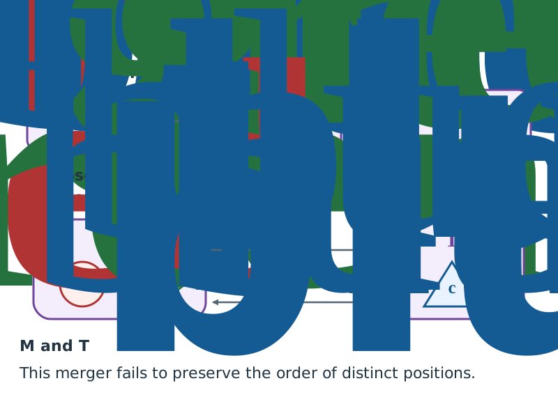
Merging by switch value breaks the order in this example
Each enclosure in the upper row contains a distinct input. Below, M combines Tred and Tgreen and contains both red cred and green cgreen. The red-to-blue relation becomes a relation from M to Tblue; the blue-to-green relation becomes a relation from Tblue to M.
M and Tblue remain distinct sets, while the relation holds in both directions. Antisymmetry of a partial order requires elements related in both directions to be identical. That condition fails here. Merging solely by the state value Closed damages the relation that distinguished the red and green inputs.
Reconstruct a usable correspondence from the cards
The cards in this example retain the counter inputs’ origins and the switch inputs’ identifiers. Card A references the red mark, Card B the blue mark, and Card C the green mark. Applying the binding rule from Section 4 pairs each input with itself and yields three separate sets containing the red, blue, and green inputs. The counter’s update rule establishes the order red, blue, green among these sets.
A numerical assignment that preserves this order gives three time representations satisfying . Reading the state of the switch input referenced by each card gives the following correspondence.
| Generated time representation | Record retaining the correspondence | Switch state read out |
|---|---|---|
| τ-red | Card A | Closed |
| τ-blue | Card B | Open |
| τ-green | Card C | Closed |
For example, specifying τ-green yields Closed through the correspondence between the input from the green mark and Card C. Specifying τ-red also yields Closed, while red and green retain distinct time representations. This constructs a function assigning Closed, Open, and Closed to their respective time representations.
The materials used in this example are internal count positions, retention of records, differences in switch states, and the coupling of identifiable inputs. We identified positions with color labels, examined the correspondences retained in the cards, constructed equivalence classes and their order, and obtained a time representation assigning real values together with a representation of object states. Because the inputs and conditions used at each stage are explicit, a failure in the construction can also be traced from its location to its consequences. If a problem is found in continuous approximation or differentiation, examine the corresponding conditions and domains of use, then repair and repeat the affected calculations.